Showing posts with label Third Year. Show all posts

Friday, 16 October 2015

PIC Microcontroller (Architecture, Features, Programming, Datasheet, Projects)

PIC MICROCONTROLLER

PIC stands for peripheral interface controller

Where as F stands for Flash it represents the type of memory used,
In 2000, Microchip introduced the PIC18 architecture.Unlike the 17 series,with a large number of device variants presently in manufacture. In contrast to earlier devices, which were more often than not programmed in assembly, C has become the predominant development language.


PIC18F4520
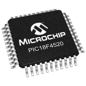
pic18f4520


Parameters of PIC18F4520 micro controller
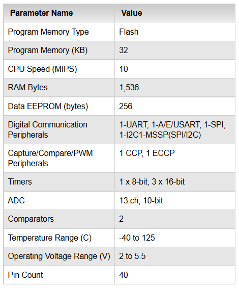
Features of PIC18f4520


Pin Diagram Of PIC18F4520

pin diagram of pic18f4520


The 18 series inherits most of the features and instructions of the 17 series, while adding a number of important new features:


PIC18 uses flash memory so that a data can be saved and erased number of times as per user requirement, not only this the battery used is used to give clock to the device.

Features of PIC micro controller

  CPU


        Up to 10 MIPS Performance at 3V
        C compiler optimized RISC architecture
        8x8 Single Cycle Hardware Multiply

  System

       
        Internal oscillator support-31 kHz to 8MHz with 4xPLL
        Fail-Safe Clock Monitor- allows safe shutdown if clock fails
        Watchdog Timer with separate RC oscillator
        Wide operating Voltage range; 2.0V to 5.5V

 nanoWatt Power Managed Modes


        Run, Idle and SLEEP modes
        Idle mode currents down to 5.8uA typical
        Sleep mode currents down to 0.1uA typical 
   

 Analog Features


        10-bit ADC, 13 channels, 100K samples per second
        Programmable Low Voltage Detection Module
        Programmable Brown-out-Reset Module
        Two Analog Comparators multiplexing 

  Peripherals

        Master Synchronous Serial Port supports SPI™ and I2C™ master and slave mode
        EUSART module including LIN bus support
        Four Timer modules
        Up to 5 PWM outputs
        Up to 2 Capture / Compare 


Advantages


  1. Small instruction set to learn and implement
  2. PIC has RISC architecture
  3. Built-in oscillator with selectable speeds
  4. Easy entry level, in-circuit programming plus in-circuit debugging PICkit units available for less than $50
  5. Inexpensive microcontrollers
  6. Wide range of interfaces including I²C, SPI, USB, USART, A/D, programmable comparators, PWM, LIN, CAN, PSP, and Ethernet
  7. Availability of processors in DIL package make them easy to handle for hobby use.


Comparison between PIC and 8051


8051- if u want a cheap controller with basic functions then 8051 will suffice . It will be of great use in your low cost college projects.

PIC- Cheap , used in refrigerators and low budget projects .

8051 and PIC need multiple clock cycles per instruction. AVR and ARM execute most instructions in a single clock cycle.

8051 and PIC have limited stack space - limited to 128 bytes for the 8051, and as little as 8 words or less for PIC. Writing a C compiler for these architectures must have been challenging, and compiler choice is limited.


Real Time Applications and Projects of PIC

1) PIC can be used to design Data Acquisition System

2)Digital clock can be implemented using PIC

3)Frequency counter are another application

4)PIC can be used as Timers, counters

5)We can design a calculator using PIC


Download Datasheet of PIC18F4520

Check out how to use PIC microcontroller using PICKit 3 or Proteus.

You can also learn how to configure DSP Processor.


Check out Complete Interview Guide For BE

Thursday, 15 October 2015

How To Configure and Run DSP Processor

Digital signal processor (DSP)


Digital signal processor (DSP) is a special type of microprocessor (or a SIP block), with its architecture optimized for the operational needs of digital signal processing.


Digital Signal Processors (DSP) take real-world signals like voice, audio, video, temperature, pressure, or position that have been digitized and then mathematically manipulate them. A DSP is designed for performing mathematical functions like "add", "subtract", "multiply" and "divide" very quickly.


C6713DSK in CCSv5

C6713DSK in CCSv5


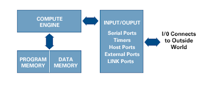
What is inside a DSP processor?


A DSP contains these key components:


  • Data Memory: Stores the information to be processed by processor
  • Program Memory: Stores the programs which the DSP will use to process data
  • Input/Output: Serves a range of functions to connect to the outside world
  • Compute Engine:It performs the math processing, accessing the program from the Program Memory and data from  Data Memory


Required Softwares

Download board support files from Spectrum Digital Website.
Unpack all files to C:\
Download CSL form TI website
Install it at C:\C6xCSL directory
Set all of jumpers on SW3 and SW1 to OFF
Connect USB then connect power

Run 6713SDKDiag.exe from C:\DSK6713\drivers to check emulator connection

Following is a step by step guide to setup a DSP processor using Non real steps CCS v5.3 DSK6713

Step 1
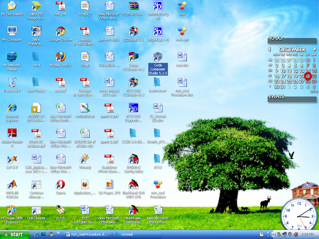
Click on ccs5.3.0 icon as shown below
How To Configure and Run DSP Processor

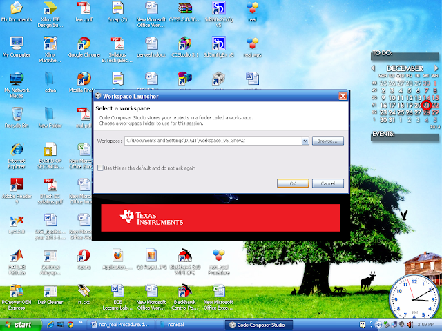
Workspace window will get open select as default or you can give your location.


How To Configure and Run DSP Processor

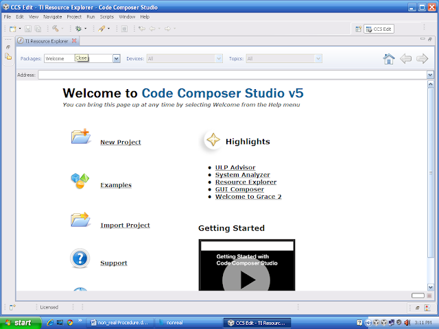
Close TI Explorer window


configure dsp processor

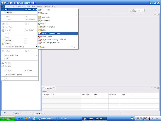
Create new target configuration
File--> new--> targetconfiguration

How To Configure and Run DSP Processor

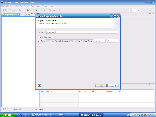
Filename: test1.ccxml


configure dsp processor

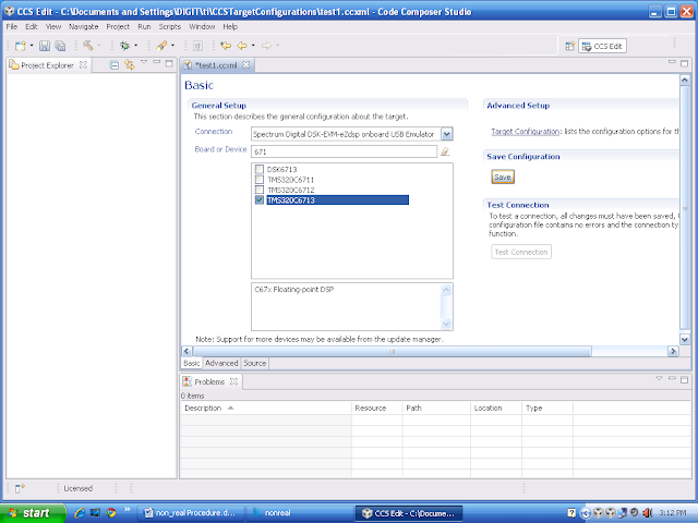
Connection: spectrum digital DSK-EVM-eZdsp on board USB emulator

Board or device: TMS320C6713

Connection: spectrum digital dsk evm ezdsp on board usb emulator Board or device: tms320c6713

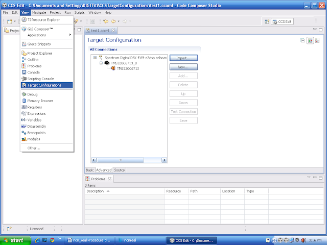
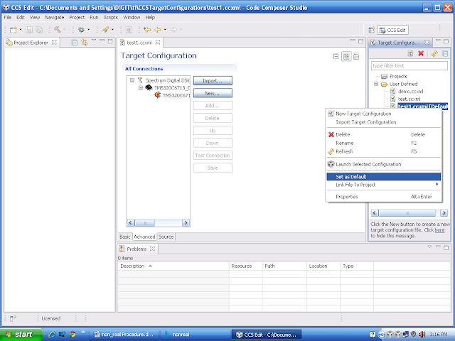
View--> targetconfiguration

target configuration

Right click on your target configuration window open at right side, set as sefault

configure dsp processor


It will jump from edit perspective to debug perspective.

Run --> connect target


configure dsp processor

Your target is connected.


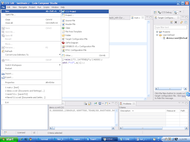
Create  new project
File-->new --> ccs project

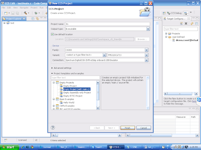
How To Configure and Run DSP Processor

Select as shown below.

dsp processor

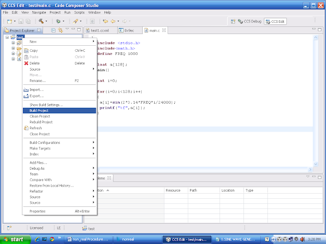
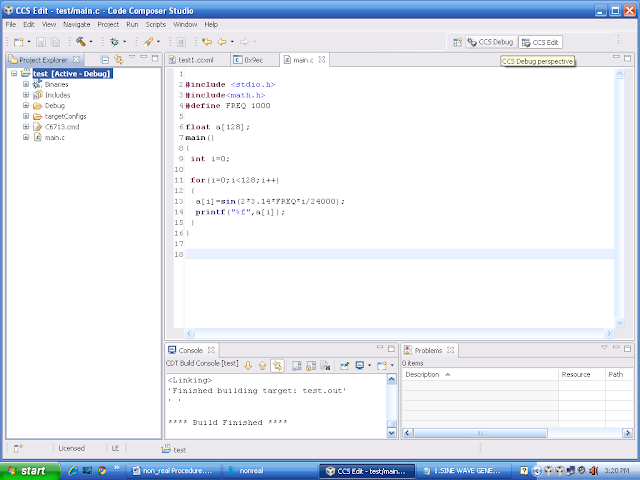
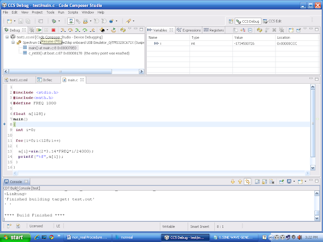
Write the code in main.c file or copy paste.
Right click on project --> build project

How To Configure and Run DSP Processor

It will generate the .out file in debug folder.
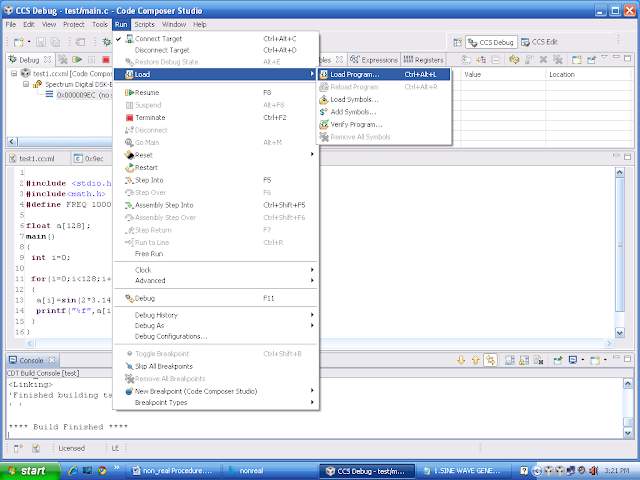
Move from edit perspective to debug prospective.
It will generate the .out file in debug folder. Move from edit perspective to debug prospective.

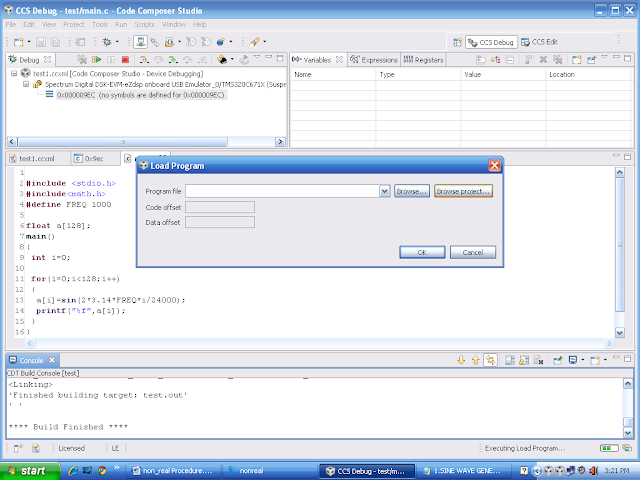
Run --> load -->load program.

configure dsp processor

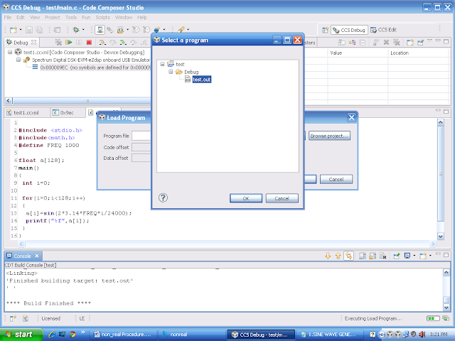
Browse project


Select Debug --> xyz.out

run dsp processor

Ok-->ok

run dsp processor

Run --> resume.

run dsp processor

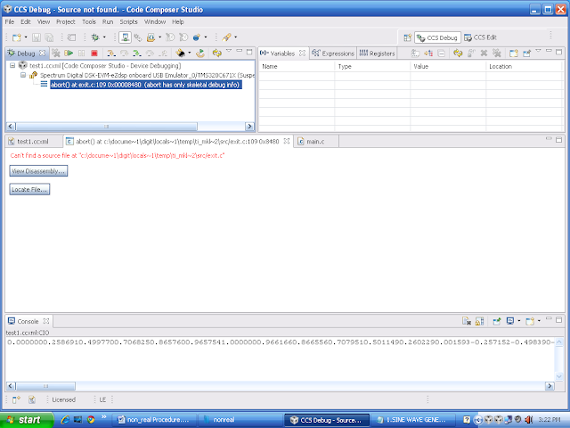
See the out put on console.

configure dsp processor

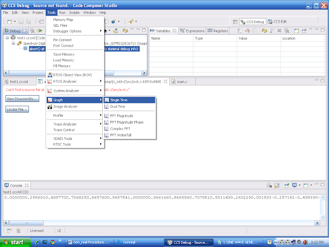
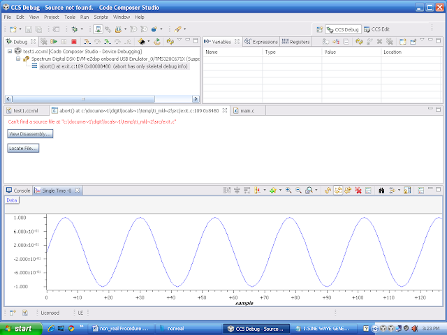
To see graph.
Tools --> graph --> single time.
Selct as shown

run dsp processor

run dsp processor

Real time

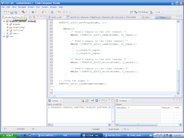
It is same like non real but you need to add BSL and CSL file.
Copy real time codec code to main.c.
run dsp processor

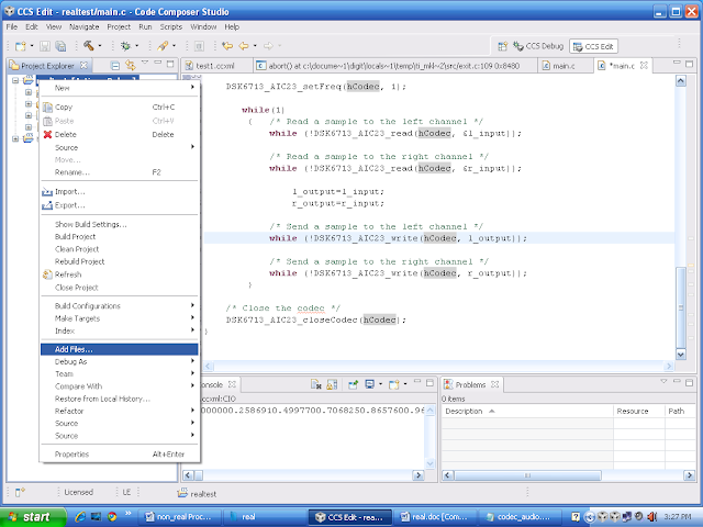
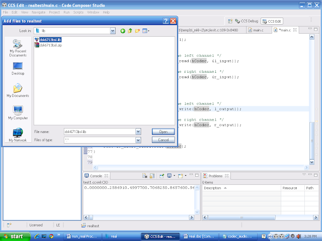
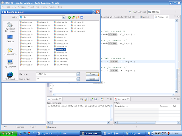
Right click on project --> add files

dsp processor

C:\CCStudio_v3.1\C6000\dsk6713\lib\dsk6713bsl.lib

run dsp processor

C:\CCStudio_v3.1\C6000\csl\lib\csl6713.lib

run a dsp processor

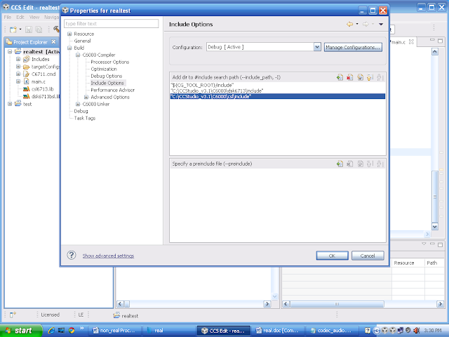
Add header file for csl and bsl.
Right click on project properties --> include option
Add dir to #include click on green colour plus sign symbol.

C:\CCStudio_v3.1\C6000\dsk6713\include.
C:\CCStudio_v3.1\C6000\csl\include.

run dsp processor


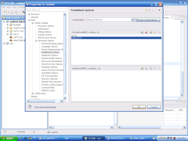
Predefined symbol -->  pre-define Name
click on green colour plus sign symbol.
Type CHIP_6713 and save.

dsp processor

Now debug the code and  load the .out file to board same like non real procedure.

Possibility error

Install again and again
Disable antivirus or uninstall


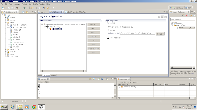
Add gel files:
CCStudio_v3.1\cc\gel\DSK6713.gel

configure dsp processor


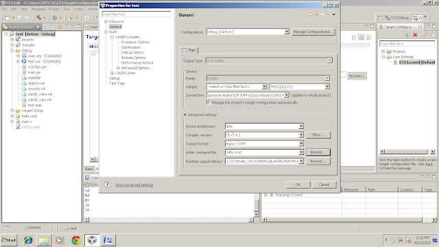
Add 
Linker command file : C:\CCStudio_v3.1\tutorial\dsk6713\hello1\hello.cmd
and
Run time support libarray: C:/CCStudio_v3.1/C6000/cgtools/lib/rts6700.lib

How To Configure and Run DSP Processor

Tuesday, 13 October 2015

Linear Convolution Matlab Program

Linear Convolution


Aim: To perform linear convolution using MATLAB

Requirements:
MATLAB 2007 and above (other version may also work but i havent tried personally)


Theory


Convolution is a formal mathematical operation, just as multiplication, addition, and integration. Addition takes two numbers and produces a third number, while convolution takes two signals and produces a third signal. Convolution is used in the mathematics of many fields, such as probability and statistics. In linear systems, convolution is used to describe the relationship between three signals of interest: the input signal, the impulse response, and the output signal.

If the input and impulse response of a system are x[n] and h[n] respectively, the convolution is given by the expression,

x[n] * h[n] = ε x[k] h[n-k]

Where k ranges between -∞ and ∞

If,

x(n) is a M- point sequence
h(n) is a N – point sequence
then, y(n) is a (M+N-1) – point sequence.

In this equation, x(k), h(n-k) and y(n) represent the input to and output from the system at time n. Here we could see that one of the inputs is shifted in time by a value every time it is multiplied with the other input signal. Linear Convolution is quite often used as a method of implementing filters of various types.


In mathematics and, in particular, functional analysis, convolution is a mathematical operation on two functions f and g, producing a third function that is typically viewed as a modified version of one of the original functions, giving the area overlap between the two functions as a function of the amount that one of the original functions is translated. Convolution is similar to cross-correlation. It has applications that include probability, statistics, computer vision, natural language processing, image and signal processing, engineering, and differential equations.

The convolution can be defined for functions on groups other than Euclidean space. For example, periodic functions, such as the discrete-time Fourier transform, can be defined on a circle and convolved by periodic convolution. A discrete convolution can be defined for functions on the set of integers. Generalizations of convolution have applications in the field of numerical analysis and numerical linear algebra, and in the design and implementation of finite impulse response filters in signal processing.


Matlab allows us to perform almost all of the digital signal processing applications on software, which makes it a lot easier to study the principles of digital signal processing and digital communication. Matlab almost performs all the operations regarding audio video and signals. One of the most important feature of matlab is that we can plot our results and observe them which is difficult manually.

Computing the inverse of the convolution operation is known as deconvolution.

x=input('Enter the first sequence - '); 
h=input('Enter the second sequence - ');
m=length(x);
n=length(h);
y=zeros(1,m+n-1);
h=[h,zeros(1,m+n-1)];
x=[x,zeros(1,m+n-1)];
cnt=0;
for i=1:1:m+n-1;
    cnt=i;
    for j=1:1:n
        y(1,cnt)=y(1,cnt)+h(j)*x(i)
        if cnt<m+n-1
            cnt=cnt+1;
        end
        
    end
end
disp (y)


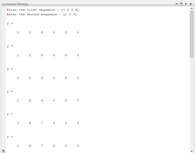
Linear Convolution

Linear convolution


Result: Throught this experiment we were able to verify linear convolution using matlab, we can verify circular convolution using linear convolution you can check below post
Here are some other programs of DSP Matlab

Discrete fourier transform
Modulo operator 
Linear Convolution 

Sunday, 11 October 2015

Discrete Fourier Transform Matlab Program (Digital Signal Processing)

Discrete Fourier Transform Matlab Program


Fourier transformation is used to decompose time series signals into frequency components each having an amplitude and phase. Using the inverse Fourier transformation the time series signal can be reconstructed from its frequency-domain representation. Fourier transformation is one of the most important concepts in digital signal processing and is not only used for estimating the spectral distribution of a signal in the frequency domain (the power spectrum). Fourier transformation is also the foundation of coherence analysis and certain types of so called surrogate signals. Finally, the Fourier transformation is implemented in many DSP (Digital Signal Processing) routines because any mathematical operation in the time domain has an equivalent operation in the frequency domain that is often computationally faster. Thus, Fourier transformation is occasionally implemented solely to speed up algorithms. Using the inverse Fourier transformation, the time-domain signal is reconstructed from its frequency domain representation.


Matlab allows us to perform almost all of the digital signal processing applications on software, which makes it a lot easier to study the principles of digital signal processing and digital communication. Matlab almost performs all the operations regarding audio video and signals. One of the most important feature of matlab is that we can plot our results and observe them which is difficult manually. Following is the program to generate a dft sequence and observe the output on the graph and verify the result manually


Comparison between FFT and DFT


The Fourier transform is important in mathematics, engineering, and the physical sciences.  Its discrete counterpart, the Discrete Fourier Transform (DFT), which is normally computed using the so-called Fast Fourier Transform (FFT), has revolutionized modern society, as it is ubiquitous in digital electronics and signal processing.  Radio astronomers are particularly avid users of Fourier transforms because Fourier transforms are key components in data processing (e.g., periodicity searches) and instruments (e.g., antennas, receivers, spectrometers), and they are the corner stores of interferometry and aperture synthesis.

%% The Program Generates DFT of a Sequence
% Equation of DFT implemented as part of assignment
% The Function takes x as discrete time sequence input from user
% N point DFT is calculated for the same sequence
% N can be default equal to length(x) or any input from user of 2^
% Syntax of calling Function from other program or command prompt
% x=input('Enter the sequence from user');
% N1=input('Enter the N Point DFT of the sequence');

function [X]=mydft(x,N1)
% if length of N point DFT given by user,
% N will be calculted for length(x)
x=input('Enter the sequence from user');
N1=input('Enter the N Point DFT of the sequence')
len=length(x);
if N1<len
    N=len;
else
    N=N1;
end
% pre allocation of Variable X: Generation of zeros Matrix
X=zeros(1,N);
%% Computation of DFT of the sequence 
% X[k]=x[n]*exp(-j*2*pi*n*k);

%X[k]=x[n]*[cos(2*pi*n*k)-j*sin(2*pi*n*k)];
%X[k]=x[n]*W  where W=exp((-j*2*pi*n*k)/N);
% The limits of k, n can varied from 1:N hence in equation (k-1), (n-1)
% being used

for k=1:N
    for n=1:N
        X(1,k)=X(1,k)+x(n)*(cos((2*pi*(k-1)*(n-1))/N)-j*(sin((2*pi*(k-1)*(n-1))/N)));
    end
end

%% The results can be verified with built in function fft
X1=fft(x,N);


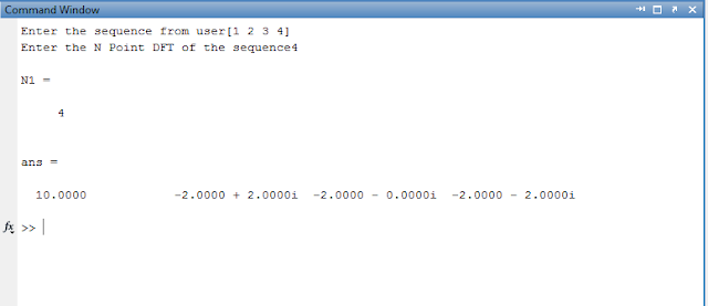
Output


Discrete fourier transform

You can directly copy paste this program in your Matlab Editor and run it, any queries and questions are welcome.
Entc Engg. Powered by Blogger.